A Variable Sampling & Acceptance Polygon Approach for Content Uniformity

We propose a method for demonstrating content uniformity in the context of variables sampling and relate this to the acceptance criteria and probability of passing the USP CU test. We demonstrate that a variable sampling plan with 99.4% coverage between 83.5% and 116.5% of label content is approximatively equivalent to (and even stricter than) the 95% probability of passing the USP test.
The views expressed in this paper are professional opinions of the authors and may not necessarily represent the position of Novartis.
To ensure the consistency of dosage units, individual batch units are controlled to achieve drug substance content within a sufficiently narrow range around the label claim. The most common test for content uniformity (CU) of dosage units is described in United States Pharmacopeia (USP) general chapter <905>.1 The USP requirements and CU acceptance values for oral solid dosage (OSD) forms (e.g., tablets and capsules) are well known and summarized in Table A, where:
AV is the acceptance value
x̄ is the mean of the samples (as percent of the label claim)
s is the standard deviation of the samples
k is the acceptability constant
If n = 10, then k = 2.4 (Stage 1)
If n = 30, then k = 2.0 (Stage 2)
The reference value M
= 98.5 if x̄ < 98.5
= 101.5 if x̄ > 101.5
= x̄ if 98.5 < x̄ < 101.5
This paper proposes a method for demonstrating CU using acceptance sampling plans and relates it to acceptance criteria and the probability of passing the USP CU test.
A variable sampling plan ensures that at least a specified proportion of a population is within a specified range with a given confidence. Variable sampling plans can be used to set acceptance criteria and support process validation or batch release. This ensures that at least a certain proportion of tablets in a batch have an assay value that falls between defined limits with a given confidence.
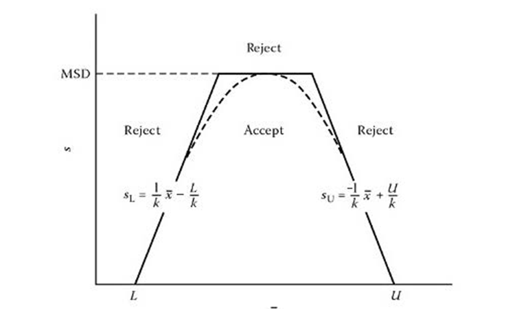
The shape of the acceptance region as a function of the mean and standard deviation of a sample can be approximated by a polygon, as shown in Figure 1. For more details, refer to Schilling.2
The acceptance polygon equation consists of two separate one-sided tolerance intervals with an upper limit on the maximum standard deviation
(MSD):
x̄ – ks > L
x̄ + ks < U
s < MSD
Where:
x̄ = sample mean
s = standard deviation
k = one-sided tolerance factor; the k value is a function of the confidence
level desired, proposed coverage, and number of samples
U = upper specification limit
L = lower specification limit
MSD = (U – L) * F, where F is a tabulated value
| Stage | Number tested | Pass if: |
|---|---|---|
| S1 | n = 10 | AV =| x̄ – M| + ks < 15 |
| S2 | n = 30 | AV =| x̄ – M| + ks < 15 |
- 1US Pharmacopeial Convention. “<905> Uniformity of Dosage Units.” December 2011. http://www.usp.org/sites/default/files/usp_pdf/EN/USPNF/2011-02-25905UNIFORMITYOFDOSAGEUNITS.pdf
- 2Schilling E.G., and D. V. Neubauer. Acceptance Sampling in Quality Control, 2nd edition. CRC Press, 2009.
The lot or batch shall be considered acceptable if the applicable k and F criteria are met.
For double-sided specifications:
1. Both (U – x̄) ∕ s and (x̄ – L) ∕ s must be ≥ k to meet the k criterion
2. s ∕ (U – L) must be ≤ F to meet the F criterion
x̄ = sample mean
s = sample standard deviation,
U = upper specification limit
L = lower specification limit
Criterion 2 can also be expressed as S ≤ smax, where Smax = (U – L) * F is the MSD. The k and F values are shown in Tables H and I for 90% or 95% confidence and 99% coverage. For any confidence and coverage values, tables can be generated as follows:
k is the critical distance and can be calculated from the noncentral t-distribution:
\( k = t^{-1}(1 - ∝, n - 1, φ) / \sqrt{n} \)
Where:
1– α = confidence level
n = sample size
\( φ = \sqrt{n}*Z_p = \text{non-centrality factor} (p = \text{coverage}) \)
F can be calculated as:
1. Find the upper tail normal area p** corresponding to zp* = k
2. Find Zp** corresponding to a normal upper tail area of p**2
3. F = 1 / (2 Zp**)
Example (in R) for n = 30 with 95% confidence and 99% coverage (from Table I):
k = qt (0.95, 29, 12.74193) / sqrt (30) = 3.063901
p** = 1 – pnorm (3.063901) = 0.001092356
Zp** = qnorm (0.001092356 / 2, lower.tail = F) = 3.265592
F = 1 / (2* 3.265592) = 0.1531116
For details see Schilling and Natrella.2 ,3
Examples
The following section shows two examples to illustrate the method. The first represents simple sampling; the second shows stratified sampling with repeated measurements per location.
Single sample
We want to demonstrate with 95% confidence that 99% of a batch assay is between 85 and 115. (We will show later that this corresponds to > 97% probability of passing the USP test with 95% confidence.)
One sample was taken at 15 locations during the process (Tables B and C). We can therefore state with 95% confidence that 99% of the batch is between 85 and 115, and that acceptance criteria for validation have been met.
Multiple samples
We want to demonstrate with 95% confidence that 99% of a batch is between 85 and 115.
Duplicate samples (j = 2) were taken from 15 locations (i = 15) for a total of 30 samples (Table D). First the within, between, and overall standard deviations were estimated by variance component analysis. This can be done easily with statistical software such as Minitab (Table E):
The associated degrees of freedom are:
- Between location: i – 1 = 14
- Within location: i (j – 1) = 15
Total was calculated using Satterthwaite approximation:
$$df_{tot}=\frac{ \left( \sigma _{T}^{2} \right) ^{2}}{\frac{ \left( \frac{ \sigma _{R}^{2}+J\ast \sigma _{L}^{2}}{J} \right) ^{2}}{ \left( I-1 \right) }+\frac{ \left( \sigma _{R}^{2} \left( 1-\frac{1}{J} \right) \right) ^{2}}{I \left( J-1 \right) }} $$
$$df_{tot}=\frac{ \left( 10.223 \right) ^{2}}{\frac{ \left( \frac{5.72+2\ast4.503}{2} \right) ^{2}}{ \left( 15-1 \right) }+\frac{ \left( 5.72 \left( 1-\frac{1}{2} \right) \right) ^{2}}{15 \left( 2-1 \right) }}=23.66 \approx 24 $$
The calculation of the acceptance test is shown in Table F. Therefore, we can state with 95% confidence that 99% of the batch is between 85 and 115 and that the acceptance criteria for validation are met. This corresponds to > 97% probability of passing the USP <905> with 95% confidence.
Acceptance Regions And OC Curves
The purpose of validation is to provide a high degree of assurance that a process will consistently produce a product that meets its specifications and quality characteristics. For the USP <905> CU test, one approach is the “Bergum method”4 (named after its inventor), which is the basis of ASTM Standard E2810.5
Our proposed alternative to this standard, based on the concepts of acceptance sampling, is easier to use and can be applied to any number of tested samples. The concept of acceptance sampling is easy to understand and easy to justify as it is standard in quality control.
Tolerance interval methodology can be used to set acceptance criteria for validation or release2 and relates to variable acceptance sampling plans. When using acceptance sampling by variables, the acceptance region can be approximated by a polygon;8 this is the so-called “k method” for double-sided specification limits.2 In this article we will link the probability of passing the USP test to the statistical confidence level and coverage of a variable sampling plan.
We will demonstrate that a variable sampling plan with 99.4% coverage between 83.5 and 116.5 is approximatively equivalent to (and even stricter than) the 95% probability of passing the USP test.
Constructing the acceptance region
USP requirements and CU acceptance criteria for OSD forms are given in Table A. For the first Stage, 10 samples are taken and an acceptance value is calculated that must be smaller than 15. If this acceptance criterion is met, the test is passed. If this acceptance criterion is not met, another 20 samples are taken and an acceptance value on the total of 30 samples is calculated. If this acceptance criterion is met the test is passed. The probability of passing the test is the combined probability of passing Stage 1 or Stage 2.
- 2 a b c
- 3Natrella, M. G., “Experimental Statistics.” National Bureau of Standards Handbook 91. August 1, 1963. http://www.keysolutionsinc.com/references/NBS%20Handbook%2091.pdf
- 4Bergum J. S., “Constructing Acceptance Limits for Multiple Stage Tests.” Drug Development and Industrial Pharmacy 16, no. 14 (1990): 2153–2166.
- 5ASTM. “Standard Practice for Demonstrating Capability to Comply with the Test for Uniformity of Dosage Units.” Standard E2810-11. www.astm.org
- 8Wallis, W. A. “Lot Quality Measured by Proportion Defective,” Acceptance Sampling–A Symposium. Washington: American Statistical Association
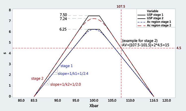
The geometric region where the USP CU test acceptance criteria are fulfilled can be represented as a function of the measured mean x̄ and standard deviations (Figure 2). Each point on the acceptance curve corresponds to an acceptance value (AV) of 15. Any point on or below the acceptance curve would pass the test (AV ≤ 15) and each point above would fail it. This acceptance region resembles the acceptance polygon of a variable sampling plan from Figure 1. Note that the standard deviation converges to zero when the mean is 83.5 or 116.5. This is why we will take 83.5 to 116.5 as our limits.
Stage 1 can be approximated with a variable sampling plan with n = 10 samples, critical distance k = 2.4, and limits between 83.5 and 116.5. Stage 2 can be approximated with a variable sampling plan with n = 30 samples, critical distance k = 2.0, and limits between 83.5 and 116.5. This is a conservative approximation, as the acceptance region is always smaller and within the USP acceptance region. (Stage 1 and Stage 2 of the USP are shown in Figure 2 as black polygons.)
All points on the polygon have an acceptance value of 15, all points inside have an acceptance value < 15, and all points above have an acceptance value > 15. Figure 2 shows an acceptance value of 15. This geometric region can be approximated by a double-variable sampling plan with Stage 1 having n = 10 samples and critical distance k = 2.4 for limits between 83.5 and 116.5, and Stage 2 having n = 30 samples and critical distance k = 2.4 for limits between 83.5 and 116.5.
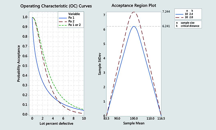
Each variable sampling plan (for n = 10 and n = 30) has an operation characteristic (OC) curve. This shows how the probability of acceptance for a lot, which is based on the sampling plan utilized and changes with the percent defective of a lot (quality). The OC curves for Stage 1 (approximated), Stage 2, and combined Stages 1 + 2 are shown in Figure 3.
| Location | Sample | Location | Sample |
|---|---|---|---|
| 1 | 98.1 | 9 | 96.9 |
| 2 | 98.6 | 10 | 98.2 |
| 3 | 101.8 | 11 | 94 |
| 4 | 94.2 | 12 | 96.7 |
| 5 | 94.5 | 13 | 96.1 |
| 6 | 96.5 | 14 | 99.7 |
| 7 | 97.4 | 15 | 102.6 |
| 8 | 92.4 |
| Name | Variable or Formula | Value |
|---|---|---|
| Number of samples | n | 15 |
| Sample average | x̄ | 97.18 |
| Sample standard deviation | s | 2.828 |
| Lower specification limits | L | 85 |
| Upper specification limits | U | 115 |
| k value (from Table I) | k | 3.52 |
| F value (from Table I) | F | 0.1351 |
| Maximum standard deviation | smax or MSD = (U – L) * F | (115-85) * 0.1351 = 4.053 |
| Lower quality index | QL = (x̄ – L) / s | (97.18-85) / 2.828 = 4.307 |
| Upper quality index | QU = (U – x̄) / s | (115-97.18) / 2.828 = 6.301 |
| Lower limit acceptance criterion Upper limit acceptance criterion smax acceptance criterion |
QL > k Q U > k s < smax |
4.307 > 3.52 (pass) 6.301 > 3.52 (pass) 2.828 < 4.053 (pass) |
| Location | Sample 1 | Sample 2 | Location | Sample 1 | Sample 2 |
|---|---|---|---|---|---|
| 1 | 100.1 | 103.0 | 9 | 99.3 | 97.3 |
| 2 | 98.9 | 101.66 | 10 | 99.8 | 104.6 |
| 3 | 99.6 | 97.9 | 11 | 102.8 | 108.6 |
| 4 | 101.8 | 100.8 | 12 | 106.8 | 103.5 |
| 5 | 102.4 | 104.6 | 13 | 102 | 102.1 |
| 6 | 98.7 | 101.1 | 14 | 96.2 | 100.5 |
| 7 | 99.2 | 99.5 | 15 | 109.1 | 102.6 |
| 8 | 99.5 | 96.5 |
The Stage 2 OC (red) is stricter than the combined Stages 1+2 OC (green). Furthermore, the green curve can only be calculated numerically. It is therefore an acceptable approximation to consider only the Stage 2 of the USP CU test. This corresponds to a critical k = 2 distance and 30 samples.
The probability of passing only Stage 2 of the USP CU test will always be smaller than the probability of passing the combined Stages 1 + 2 test, as seen when comparing the red to the green curve in Figure 3.
Characterizing the USP CU test based on the probability of passing Stage 2 only, therefore, is a conservative but valid approximation. Furthermore, the combined Stages 1 + 2 can only be computed numerically while the red OC has an analytical solution and can be described by the noncentral t distribution.
P (pass stage 2) = 1 – pt (2 * sqrt (30), 29, qnorm (1 – LotFractionDefective) * sqrt (30))
Example: For 0.6% tablets outside the 83.5 to 116.5 interval, the probability to pass the USP Stage 2 is:
1 – pt (2 * sqrt (30), 29, qnorm (1 – 0.006) * sqrt (30)) = 0.9493999 ≈ 0.95
This establishes a correspondence between the probability of passing the Stage 2 USP CU test (95%) and the proportion of samples inside the 83.5–116.5 interval (99.403%). The 95% probability of passing combined Stages 1 + 2, computed numerically, is 99.34. The probability of passing Stage 2 or the combined Stages 1 + 2 is fairly close in the upper domain of the OC curve. The probability of passing the USP versus the coverage between 83.5 to 116.5 is given in Table G.
| Source | Variance components | % total | SD |
|---|---|---|---|
| Location | 4.503 | 44.05 | 2.122 |
| Error | 5.720 | 55.95 | 2.392 |
| Total | 10.223 | 3.197 |
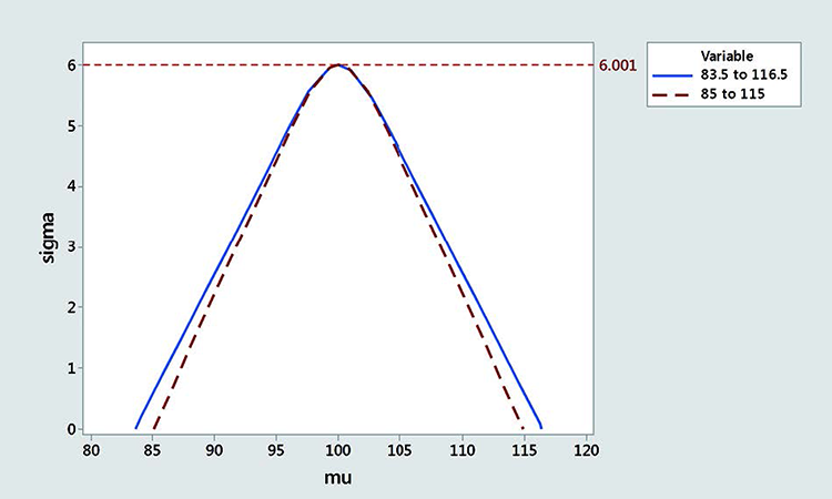
Figure 4 shows rescaled acceptance regions for 95% probability passing the USP with 83.5 to 116.5 limits and 85 to 115 limits (100% confidence for infinite number of samples). The acceptance region is smaller with the narrower border, especially when the mean is close to the border.
Since the real mean and standard deviation are unknown but estimated from a finite number of samples, we need to add a confidence level (typically 90 or 95% in cases of process validation).
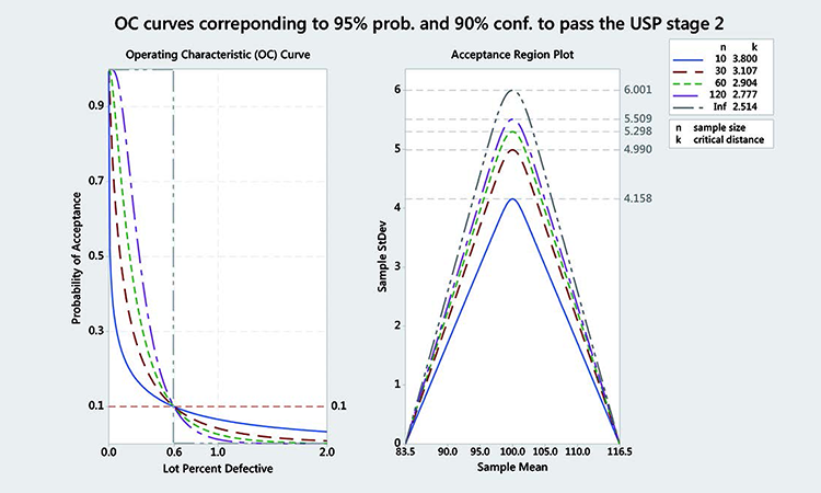
Figure 5 shows OC curves corresponding to 95% probability and 90% confidence to pass the USP Stage 2 for various numbers of samples. We can clearly see that this corresponds to a variable sampling plan with a rejectable quality level (β = 10%) at 0.6% lot percent defectives. In other words, a batch with 0.6% points outside the 83.5 to 116.5 interval (or 99.4% inside) has a 90% chance of being rejected (or 10% chance of being accepted).
The critical distance k and MSD for varying numbers of samples and 99.4% coverage between 83.5 and 116.5 (corresponding to > 95% of probability of passing the USP) are given in Tables J and K for 90% and 95% confidence.
These acceptance criteria provide an alternative to the ASTM approach by simply employing variables sampling plans.
| Name | Formula | Value |
|---|---|---|
| Number of samples | ≈ dftot | 24.0 |
| Sample average | x̄ | 101.35 |
| Sample standard deviation | s | 3.197 |
| Lower specification limits | L | 85.0 |
| Upper specification limits | U | 115.0 |
| k value (from Table I) | k | 3.181 |
| F value (from Table I) | F | 0.1481 |
| Maximum standard deviation | smax or MSD = (U – L) * F | (115 – 85) * 0.1481 = 4.443 |
| Lower quality index | QL = (x̄ – L) / s | (101.35 – 85) / 3.197 = 5.514 |
| Upper quality index | QU = (U – x̄) / s | (115 – 101.35) / 3.197 = 4.270 |
| Lower limit acceptance criterion Upper limit acceptance criterion smax acceptance criterion |
QL > k QU > k s < smax |
5.514 > 3.181 (pass) 4.270 > 3.181 (pass) 3.197 < 4.443 (pass) |
Matching The Acceptance Region
Some practitioners might argue that the range from 83.5 to 116.5 used by current USP is too large. In the following example, we rescaled the acceptance criteria to 85–115 by matching the acceptance region at the MSD. We previously shown that 99.403% coverage between 83.5 and 116.5 corresponds to more than 95% probability to pass the USP test when the number of samples is infinite. This corresponds to a critical distance k = 2.514 and MSD = 6.001. When we are on target with a mean at 100 and a standard deviation of 6.001, the proportion inside the 85–115 interval is 98.76%, which would be the new coverage. The corresponding k value, the left tailed quantile of normal distribution corresponding to 98.76% coverage, is 2.243. Table L gives the coverage between 85 and 115 for various probabilities of passing the USP.
Note that the rescaled acceptance region is always more conservative than the original one between 83.5 and 116.5, especially when the mean is close to the limit. Figure 4 shows the acceptance regions for 83.5–116.5 and 85–115 for an MSD of 6.001.
Table L shows a few interesting test properties:
- 96% coverage between 85% to 115% and 50% confidence corresponds approximately to 50% probability to pass the USP test with 50% confidence. This could be a minimal requirement for releasing batches and could be used, for instance, in PAT application when more than 30 samples are taken.
- 99% coverage between 85% to 115% corresponds approximately to 97% probability to pass the USP test. The confidence is typically chosen at 90% or 95%, since round numbers that are easy to justify and acceptance tables with 99% percent coverage are readily available.
Discussion
Variable sampling vs. ASTM E2810 Bergum4 published a method for constructing acceptance limits that relate directly to the probability of passing the USP test. These acceptance limits are defined to provide, with a confidence level (1 – α), a stated probability (P) of passing the USP test. This approach was incorporated in the ASTM Standard E2810.5
| Probability Passing USP Test |
Stage 1 (n = 10) exact | Stage 2 (n = 30) exact | Stages 1 + 2 (n = 30) numeric | ||||||
|---|---|---|---|---|---|---|---|---|---|
| Cov % (83.5–116.5) |
k | MDS | Cov % (83.5-116.5) |
k | MDS | Cov % (83.5-116.5) |
k | MDS | |
| 99 | 99.995 | 3.898 | 4.061 | 99.69 | 2.741 | 5.571 | 99.67 | 2.716 | 5.616 |
| 98 | 99.989 | 3.705 | 4.256 | 99.60 | 2.65 | 5.736 | 99.56 | 2.617 | 5.798 |
| 97 | 99.983 | 3.583 | 4.388 | 99.52 | 2.592 | 5.846 | 99.48 | 2.559 | 5.911 |
| 96 | 99.976 | 3.492 | 4.492 | 99.46 | 2.549 | 5.931 | 99.4 | 2.515 | 6 |
| 95 | 99.969 | 3.419 | 4.58 | 99.40 | 2.514 | 6.001 | 99.34 | 2.479 | 6.074 |
| 90 | 99.923 | 3.168 | 4.904 | 99.17 | 2.394 | 6.254 | 99.07 | 2.355 | 6.341 |
| 85 | 99.866 | 3.001 | 5.146 | 98.97 | 2.314 | 6.435 | 98.84 | 2.271 | 6.536 |
| 80 | 99.795 | 2.87 | 5.353 | 98.78 | 2.25 | 6.585 | 98.62 | 2.204 | 6.698 |
| 75 | 99.709 | 2.758 | 5.542 | 98.60 | 2.196 | 6.718 | 98.41 | 2.147 | 6.843 |
| 70 | 99.607 | 2.658 | 5.721 | 98.41 | 2.147 | 6.842 | 98.19 | 2.095 | 6.98 |
| 65 | 99.487 | 2.567 | 5.896 | 98.22 | 2.102 | 6.96 | 97.97 | 2.047 | 7.111 |
| 60 | 99.344 | 2.48 | 6.07 | 98.03 | 2.06 | 7.075 | 97.73 | 2.001 | 7.241 |
| 55 | 99.175 | 2.397 | 6.246 | 97.83 | 2.019 | 7.19 | 97.48 | 1.957 | 7.371 |
| 50 | 98.973 | 2.316 | 6.429 | 97.61 | 1.979 | 7.306 | 97.21 | 1.913 | 7.504 |
Table H (PDF) represents 90% confidence that 99% of population is between limits.
Table I (PDF) represents 95% confidence that 99% of population is between limits.
While our variable sampling plan and the ASTM approach have similarities and fulfill the same purpose, the variable sampling plan has several advantages, in our view:
- An acceptance polygon is easy to calculate and is defined by just two numbers: the critical distance k and the MSD. There is no need for computer-generated acceptance tables as with the ASTM method. Acceptance criteria can easily be derived for any sample size.
- Our generalized approach relates the probability of passing the CU directly to the distribution of the batch and the USP. This is less abstract than the ASTM and allows a better understanding of the process.
Variable sampling vs. tolerance intervals
Tolerance intervals, another alternative to the ASTM E2810, have recently been discussed in the literature.7 Bergum6 proposed a double-sided tolerance interval method and a coverage of 98.58% between 85% and 115% corresponding to 95% probability of passing the USP. When rescaling our results for 95% probability of passing the USP Stage 2 or the combined Stages 1 + 2 to an interval between 85% and 115%, we found coverages of 98.76% and 98.64%, respectively—fairly close to Bergum´s value of 98.58%. The value of 98.76% was derived analytically, while the values of 98.64% or 98.58% (combined Stages 1 + 2) are based on numeric simulations.
Bergum6 showed that the shape of the OC curve is very strongly dependent on the position of the mean, while in our work it is not. This is because Bergum’s OC curve calculations are based on an 85%–115% range, while the USP test was conceived with an 83.5%–116.5% limit (Figure 2). Bergum also used the USP acceptance regions (black polygon in Figure 2), while we used the more conservative acceptance region of a variable sampling plan that best matches the USP.
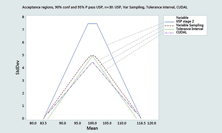
In Figure 6, we compared different acceptance regions corresponding to 95% probability and 90% confidence to pass the USP for n = 30 samples. We compared the content uniformity and dissolution acceptance limit (CUDAL)/ASTM acceptance region, a variable sampling plan with critical distance k = 3.107 corresponding to 99.4 coverage between 83.5 and 116.5, and a double-sided tolerance interval corresponding to 98.58% coverage between 85 and 115. For comparison, the acceptance region corresponding to USP Stage 2 is also given.6
Differences in shape between these acceptance regions are apparent. The acceptance region calculated by CUDAL/ASTM E2810 is the narrowest, arising from the very conservative way the confidence limits are calculated using Lindgren´s simultaneous confidence region.4 This acceptance region has a triangular shape and converges to zero at 83.5 and 116.5, like the USP test. Bergum’s tolerance interval approach and our variable sampling approach nearly match at the Smax. The tolerance interval approach is more restrictive, however, with a triangular acceptance region, while the variable sampling plan acceptance region is elliptical (can be approximated by a trapezoidal polygon) and larger.
| n | k | MSD | n | k | MSD | n | k | F | n | k | MSD |
|---|---|---|---|---|---|---|---|---|---|---|---|
| 10 | 3.8 | 4.158 | 40 | 3.01 | 5.133 | 70 | 2.871 | 5.351 | 100 | 2.805 | 5.46 |
| 11 | 3.705 | 4.255 | 41 | 3.003 | 5.144 | 71 | 2.868 | 5.356 | 101 | 2.804 | 5.463 |
| 12 | 3.627 | 4.339 | 42 | 2.996 | 5.154 | 72 | 2.865 | 5.361 | 102 | 2.802 | 5.466 |
| 13 | 3.562 | 4.412 | 43 | 2.989 | 5.165 | 73 | 2.862 | 5.365 | 103 | 2.801 | 5.468 |
| 14 | 3.506 | 4.476 | 44 | 2.982 | 5.175 | 74 | 2.86 | 5.37 | 104 | 2.799 | 5.471 |
| 15 | 3.457 | 4.533 | 45 | 2.976 | 5.184 | 75 | 2.857 | 5.374 | 105 | 2.798 | 5.474 |
| 16 | 3.415 | 4.584 | 46 | 2.97 | 5.194 | 76 | 2.854 | 5.378 | 106 | 2.796 | 5.476 |
| 17 | 3.377 | 4.631 | 47 | 2.964 | 5.203 | 77 | 2.852 | 5.383 | 107 | 2.795 | 5.479 |
| 18 | 3.343 | 4.673 | 48 | 2.959 | 5.211 | 78 | 2.849 | 5.387 | 108 | 2.793 | 5.481 |
| 19 | 3.313 | 4.711 | 49 | 2.953 | 5.22 | 79 | 2.847 | 5.391 | 109 | 2.792 | 5.484 |
| 20 | 3.286 | 4.746 | 50 | 2.948 | 5.228 | 80 | 2.845 | 5.395 | 110 | 2.79 | 5.486 |
| 21 | 3.261 | 4.779 | 51 | 2.943 | 5.236 | 81 | 2.842 | 5.398 | 111 | 2.789 | 5.488 |
| 22 | 3.238 | 4.809 | 52 | 2.938 | 5.244 | 82 | 2.84 | 5.402 | 112 | 2.788 | 5.491 |
| 23 | 3.217 | 4.837 | 53 | 2.933 | 5.251 | 83 | 2.838 | 5.406 | 113 | 2.786 | 5.493 |
| 24 | 3.198 | 4.863 | 54 | 2.929 | 5.258 | 84 | 2.836 | 5.41 | 114 | 2.785 | 5.495 |
| 25 | 3.18 | 4.888 | 55 | 2.924 | 5.265 | 85 | 2.833 | 5.413 | 115 | 2.784 | 5.498 |
| 26 | 3.163 | 4.911 | 56 | 2.92 | 5.272 | 86 | 2.831 | 5.417 | 116 | 2.782 | 5.5 |
| 27 | 3.148 | 4.933 | 57 | 2.916 | 5.279 | 87 | 2.829 | 5.42 | 117 | 2.781 | 5.502 |
| 28 | 3.133 | 4.953 | 58 | 2.912 | 5.285 | 88 | 2.827 | 5.424 | 118 | 2.78 | 5.504 |
| 29 | 3.12 | 4.972 | 59 | 2.908 | 5.292 | 89 | 2.825 | 5.427 | 119 | 2.779 | 5.506 |
| 30 | 3.107 | 4.991 | 60 | 2.904 | 5.298 | 90 | 2.823 | 5.43 | 120 | 2.777 | 5.508 |
| 31 | 3.095 | 5.008 | 61 | 2.9 | 5.304 | 91 | 2.821 | 5.433 | 150 | 2.747 | 5.561 |
| 32 | 3.083 | 5.025 | 62 | 2.897 | 5.31 | 92 | 2.819 | 5.437 | 200 | 2.713 | 5.621 |
| 33 | 3.072 | 5.04 | 63 | 2.893 | 5.315 | 93 | 2.818 | 5.44 | 300 | 2.675 | 5.691 |
| 34 | 3.062 | 5.055 | 64 | 2.89 | 5.321 | 94 | 2.816 | 5.443 | 400 | 2.652 | 5.733 |
| 35 | 3.052 | 5.07 | 65 | 2.886 | 5.326 | 95 | 2.814 | 5.446 | 500 | 2.637 | 5.762 |
| 36 | 3.043 | 5.083 | 66 | 2.883 | 5.331 | 96 | 2.812 | 5.449 | 1,000 | 2.599 | 5.832 |
| 37 | 3.034 | 5.096 | 67 | 2.88 | 5.337 | 97 | 2.81 | 5.452 | 2,000 | 2.574 | 5.882 |
| 38 | 3.026 | 5.109 | 68 | 2.877 | 5.342 | 98 | 2.809 | 5.455 | 3,000 | 2.563 | 5.904 |
| 39 | 3.018 | 5.121 | 69 | 2.874 | 5.347 | 99 | 2.807 | 5.457 | Inf | 2.514 | 6.001 |
| n | k | MSD | n | k | MSD | n | k | F | n | k | MSD |
|---|---|---|---|---|---|---|---|---|---|---|---|
| 10 | 4.28 | 3.723 | 40 | 3.167 | 4.905 | 70 | 2.98 | 5.178 | 100 | 2.894 | 5.314 |
| 11 | 4.142 | 3.839 | 41 | 3.157 | 4.919 | 71 | 2.976 | 5.184 | 101 | 2.892 | 5.318 |
| 12 | 4.029 | 3.939 | 42 | 3.148 | 4.933 | 72 | 2.973 | 5.19 | 102 | 2.889 | 5.321 |
| 13 | 3.935 | 4.026 | 43 | 3.139 | 4.945 | 73 | 2.969 | 5.195 | 103 | 2.887 | 5.325 |
| 14 | 3.855 | 4.103 | 44 | 3.13 | 4.958 | 74 | 2.965 | 5.201 | 104 | 2.885 | 5.328 |
| 15 | 3.786 | 4.172 | 45 | 3.121 | 4.97 | 75 | 2.962 | 5.206 | 105 | 2.883 | 5.331 |
| 16 | 3.726 | 4.234 | 46 | 3.113 | 4.981 | 76 | 2.958 | 5.212 | 106 | 2.881 | 5.334 |
| 17 | 3.673 | 4.29 | 47 | 3.105 | 4.992 | 77 | 2.955 | 5.217 | 107 | 2.879 | 5.337 |
| 18 | 3.626 | 4.341 | 48 | 3.098 | 5.003 | 78 | 2.952 | 5.222 | 108 | 2.877 | 5.341 |
| 19 | 3.583 | 4.388 | 49 | 3.091 | 5.014 | 79 | 2.949 | 5.227 | 109 | 2.876 | 5.344 |
| 20 | 3.545 | 4.431 | 50 | 3.084 | 5.024 | 80 | 2.945 | 5.232 | 110 | 2.874 | 5.347 |
| 21 | 3.511 | 4.47 | 51 | 3.077 | 5.034 | 81 | 2.942 | 5.237 | 111 | 2.872 | 5.35 |
| 22 | 3.479 | 4.507 | 52 | 3.07 | 5.043 | 82 | 2.939 | 5.242 | 112 | 2.87 | 5.353 |
| 23 | 3.45 | 4.542 | 53 | 3.064 | 5.053 | 83 | 2.936 | 5.246 | 113 | 2.868 | 5.356 |
| 24 | 3.424 | 4.574 | 54 | 3.058 | 5.062 | 84 | 2.933 | 5.251 | 114 | 2.867 | 5.358 |
| 25 | 3.399 | 4.604 | 55 | 3.052 | 5.07 | 85 | 2.931 | 5.255 | 115 | 2.865 | 5.361 |
| 26 | 3.376 | 4.632 | 56 | 3.046 | 5.079 | 86 | 2.928 | 5.26 | 116 | 2.863 | 5.364 |
| 27 | 3.355 | 4.659 | 57 | 3.04 | 5.087 | 87 | 2.925 | 5.264 | 117 | 2.861 | 5.367 |
| 28 | 3.335 | 4.684 | 58 | 3.035 | 5.095 | 88 | 2.922 | 5.268 | 118 | 2.86 | 5.37 |
| 29 | 3.316 | 4.708 | 59 | 3.03 | 5.103 | 89 | 2.92 | 5.273 | 119 | 2.858 | 5.372 |
| 30 | 3.298 | 4.73 | 60 | 3.025 | 5.111 | 90 | 2.917 | 5.277 | 120 | 2.857 | 5.375 |
| 31 | 3.282 | 4.752 | 61 | 3.02 | 5.118 | 91 | 2.915 | 5.281 | 150 | 2.816 | 5.442 |
| 32 | 3.266 | 4.772 | 62 | 3.015 | 5.126 | 92 | 2.912 | 5.285 | 200 | 2.772 | 5.517 |
| 33 | 3.252 | 4.791 | 63 | 3.01 | 5.133 | 93 | 2.91 | 5.289 | 300 | 2.723 | 5.604 |
| 34 | 3.238 | 4.81 | 64 | 3.006 | 5.14 | 94 | 2.907 | 5.292 | 400 | 2.693 | 5.658 |
| 35 | 3.224 | 4.827 | 65 | 3.001 | 5.146 | 95 | 2.905 | 5.296 | 500 | 2.673 | 5.695 |
| 36 | 3.212 | 4.844 | 66 | 2.997 | 5.153 | 96 | 2.903 | 5.3 | 1,000 | 2.624 | 5.785 |
| 37 | 3.2 | 4.861 | 67 | 2.992 | 5.159 | 97 | 2.9 | 5.304 | 2,000 | 2.591 | 5.848 |
| 38 | 3.189 | 4.876 | 68 | 2.988 | 5.166 | 98 | 2.898 | 5.307 | 3,000 | 2.577 | 5.877 |
| 39 | 3.178 | 4.891 | 69 | 2.984 | 5.172 | 99 | 2.896 | 5.311 | Inf | 2.514 | 6.001 |
Conclusion
We derived a relationship between the probability of passing the USP and a variable sampling plan ensuring with a certain confidence that a certain proportion of values are between certain limits. The limits of the USP CU are between 83.5 and 116.5%, but narrower limits like 85% to 115% (or others) are also possible.
To assess the capability of intrabatch CU within process validation, different confidence and coverage values and interval ranges (corresponding to various probabilities of passing the USP test) are possible. We suggest taking typically 90% or 95% confidence and 99.4% coverage between 83.5% and 116.5%. This most closely matches 95% probability of passing the USP CU. A more conservative value would be 99% of tablets between 85 and 115. This corresponds to > 97% probability to pass the USP.
We recommend taking 30 samples, with 15 being a minimum. The smaller the sample size, the higher the risk to fail validation as the size of the acceptance region shrinks with a decreasing number of samples.
| Probability of passing USP Stage 2 | Smax | k = 1/slope 83.5–116.5 | Coverage %83.5–116.5 | k = 1/slope 85–115 |
Coverage % 85–115 |
|---|---|---|---|---|---|
| 99 | 5.571 | 2.741 | 99.69 | 2.453 | 99.29 |
| 98 | 5.736 | 2.65 | 99.6 | 2.369 | 99.11 |
| 97 | 5.846 | 2.592 | 99.52 | 2.316 | 98.97 |
| 96 | 5.931 | 2.549 | 99.46 | 2.276 | 98.86 |
| 95 | 6.001 | 2.514 | 99.4 | 2.244 | 98.76 |
| 90 | 6.254 | 2.394 | 99.17 | 2.133 | 98.35 |
| 85 | 6.435 | 2.314 | 98.97 | 2.059 | 98.02 |
| 80 | 6.585 | 2.25 | 98.78 | 2 | 97.73 |
| 75 | 6.718 | 2.196 | 98.6 | 1.95 | 97.44 |
| 70 | 6.842 | 2.147 | 98.41 | 1.906 | 97.16 |
| 65 | 6.96 | 2.102 | 98.22 | 1.864 | 96.89 |
| 60 | 7.075 | 2.06 | 98.03 | 1.825 | 96.6 |
| 55 | 7.19 | 2.019 | 97.83 | 1.787 | 96.3 |
| 50 | 7.306 | 1.979 | 97.61 | 1.75 | 95.99 |
This paper provides a clear methodology to assess intrabatch capability based on total observed variability. Further controls on location means stratified sampling can also be pursued to protect against undesirable within batch trends that cannot be controlled by capability assessment alone.Another advantage of this method is that it is also easily applicable when there are several samples per location.
Acknowledgments
The authors thank Andrea Kramer, Head of Manufacturing Science and Technology at Novartis Wehr, Germany, for her continuous support during the preparation of this work. Many thanks also to James Crichton, Abe Germansderfer, and all nonclinical statisticians from the Novartis statistics network for their helpful discussions and comments.
- 4 a b
- 5
- 7De los Santos P.A., L. B. Pfahler, K. E. Vukovinsky, J. Liu, and B. Harrington. “Performance Characteristics and Alternative Approaches for the ASTM E2709/2810 (CUDAL) Method for Ensuring That a Product Meets USP <905> Uniformity of Dosage Units.” Pharmaceutical Engineering 36, no. 5 (October 2015).
- 6 a b Bergum J. S. “Tolerance interval Alternative to ASTM E2709/E2810 Methodology.” Pharmaceutical Engineering 35, no. 6 (December 2015).