Using CFD Multiphase Modeling to Predict Bioreactor Performance
Computational fluid dynamics (CFD) can reduce or eliminate the need to perform bioreactor scale-up studies because full-scale manufacturing bioreactors can be simulated to predict performance. This article discusses the use of computational fluid dynamics for that purpose, to predict the performance of a manufacturing-scale bioreactor under various operating conditions.
Parametric studies on process conditions provide valuable insight for early-stage bioreactor design and process development. The advantage of computational fluid dynamics is that it enables rapid and cost-effective simulation of various conditions and provides detailed visual data that can complement or exceed experimental methods. Furthermore, individual parameters within CFD simulations can be varied with precision to facilitate design optimization with results interpreted at a level that is often masked by natural variation in physical testing.
The goal of this article is to provide a method for simulating and analyzing impeller mixing and gas sparging in a bioreactor using multiphase computational fluid dynamics modeling. In particular, the oxygen transfer rate, kLa, is the primary performance parameter of interest, and to ensure the validity of the solutions, a mesh-independent computational fluid dynamics model is benchmarked against an experimentally determined kLa. Operating parameters (i.e., impeller speed, gas sparge rate) for the mesh-independent and benchmarked computational fluid dynamics models are then changed, and a comparison is made between the computational fluid dynamics model prediction and experimental data. One bioreactor computational fluid dynamics model is created and solved to simulate three different operating conditions. The model can then be used for further parametric studies for the purpose of design optimization, specifically for changing operating conditions such as sparge gas flow rate and impeller speed. These simulations were performed with ANSYS CFX version 2019R3. The method presented here is not limited to oxygen transfer and may also be used for other species (e.g., CO2 stripping) undergoing liquid and gas mass transfer.
Methodology
Our modeling approach incorporated the homogeneous multiple size group (MUSIG) model to account for multiple sizes of bubbles, bubble breakup, and bubble coalescence. This model assigns the same velocity to the different bubble size groups in the bioreactor. This essentially means that small bubbles will have the same velocity as large bubbles even though, in reality, different sizes of bubbles have different terminal rise velocities. For air bubbles in a water-type liquid environment, the MUSIG model is appropriate for bubble sizes in the approximately 1 mm to 17 mm range.
Using the formulas from Talaia1 and liquid and gas densities of 993.5 kg/m3 and 1.65 kg/m3, respectively, the terminal rise velocity for air bubbles ranging from 1 mm to 17 mm is 0.15 m/s (1 mm) to 0.61 m/s (17 mm). The terminal velocity of the largest bubble can be approximately four times that of the smallest bubble. In practice, for these gas-sparged vessel mixing setups, most bubbles cluster within a tighter size range than the size range in which the MUSIG model applies. In addition, other studies have compared the inhomogeneous and homogeneous MUSIG models for vessel mixing with the homogeneous model, providing good results against experimental data.2
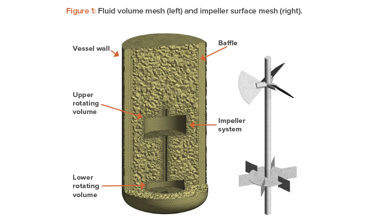
We made four sets of simulations, with each set containing three different operating conditions, for a total of 12 simulations. Different setups were used to determine which options predict better results. The different setups used are summarized as follows:
- Setup 1: Compressible fluid for gas phase, second-order Rhie-Chow option for pressure-velocity coupling
- Setup 2: Incompressible fluid for gas phase, second-order Rhie-Chow option for pressure-velocity coupling
- Setup 3: Incompressible fluid for gas phase, fourth-order Rhie-Chow option for pressure-velocity coupling
- Setup 4: Incompressible fluid for gas phase, fourth-order Rhie-Chow option for pressure-velocity coupling, virtual mass, and enhanced turbulence using the Sato-enhanced eddy viscosity model
This article illustrates which setup provides better agreement with experimental data.
Oxygen Mass Transfer Rate
There are several theories for calculating the oxygen mass transfer coefficient, kL. Sarkar and coauthors3 used the following equation:
\(\text{Equation 1:}\ k_L=\frac{2}{ \sqrt{\pi} }\sqrt{D_0}\left(\frac{\epsilon_L\ \rho_L}{\mu_L} \right)^{1/4} \)
where D0 is the oxygen diffusivity in water, m2/s; \(\epsilon_L\) is the liquid turbulent eddy dissipation, m2/s3; \(\mu_L) \) is the liquid viscosity, Pa⋅s; and \(\rho_L) \) is the liquid density, kg/m3.
Others have used different mass transfer formulas, as shown in Equations 2, 3, and 4:4
\(\text{Equation 2:}\ k_L=\frac{2}{ \sqrt{\pi} }\sqrt{D_0}\left(\frac{\epsilon_L\ \rho_L}{\mu_L} \right)^{1/4} \)
\(\text{Equation 3:}\ k_L=0.4\sqrt{D_0}\left(\frac{\epsilon_L\ \rho_L}{\mu_L} \right)^{1/4} \)
\(\text{Equation 4:}\ k_L=0.5\sqrt{D_0}\left(\frac{\epsilon_L\ \rho_L}{\mu_L} \right)^{1/4} \)
Petitti and colleagues5 state that the constant in front of \(\sqrt{D_0}\left(\frac{\epsilon_L\ \rho_L}{\mu_L} \right)^{1/4} \) is sometimes replaced with one that is tuned with experiments; this was the approach taken in our study. In Table 3 of Ranganathan and Sivaraman,2 it is the eddy cell theory, with a constant of 0.4, that provided the best kL estimate against experimental data. We initially used this same 0.4 constant in our study to solve the models; then, the constant was adjusted so computational fluid dynamics kLa (see equation 5) matched experimental data for the benchmarking case (for each of the four different setups). The kLa constant for the other two simulations was then updated to that of the benchmarked kLa constant, and the percent difference between computational fluid dynamics and experimental kLa was determined.
The volume-averaged mass transfer coefficient is the product of kL and the interfacial area, a, as shown in equation 5:
\(\text{Equation 5:}\ k_La= k_L\frac{^{6\alpha}g}{d_{32}} \)
where \(^{6\alpha}g \) is the gas volume fraction and d32 is the Sauter diameter, m.
Modeling Approach
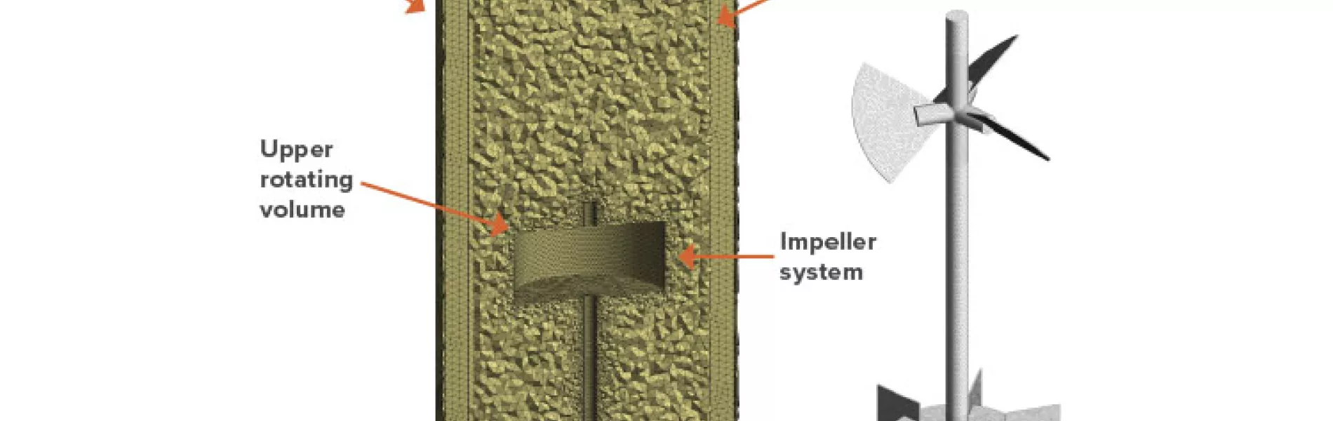
The technique we used to model the rotating impellers is a frozen rotor method. The frozen rotor method keeps the impeller static and changes the frame of reference to capture the rotating impeller physics. This technique requires that the fluid volume within the vessel be divided in the following way:
- A fluid volume that is assigned a rotation speed and encompasses the impeller (typically, a cylindrical volume). For multiple impellers, a single rotating volume can encompass all the impellers or several rotating volumes can be used, one for each impeller (see Figure 1).
- A static volume for the vessel, which encompasses the vessel wall, free surface, air sparger, part of the impeller shaft, and baffles.
Assumptions
The following assumptions were made in our study:
- The liquid was assumed to be water and exhibit water-like properties at 37°C (98.6°F), actual bioreactor temperature.
- The air was assumed to be injected at a temperature of 26.7°C (80°F) and was modeled as an ideal gas (varying density) for one set of simulations and as an incompressible gas (constant density) for the other set of simulations.
- As is common practice with these types of simulations, small components such as bolts and side ports were not modeled because these components were assumed to only affect the flow locally and have an insignificant influence on the overall flow structure. In addition, modeling of small components requires the mesh density to increase, thereby needlessly increasing the solver time.
- The free surface was modeled as a horizontal degassing surface; thus, surface effects due to gravity were ignored. This assumption is reasonable when the vessel contains baffles because they eliminate any large rotating vortex structure that may develop at the center of the vessel due to the impeller(s). The degassing surface acts as a free-slip condition for liquid and allows gas to escape the surface.
Selected Conditions
We used the following conditions for this study:
- The following properties were used:
- A liquid density of 993.5 kg/m3
- A liquid viscosity of 0.0007 Pa⋅s
- A liquid surface tension of 0.07 N/m
- An air-to-water oxygen diffusion coefficient of 3.0 × 10⁻⁵ cm2/s
- A total of 10 bubble size groups were used for the population balance model based on an equal diameter distribution (i.e., bubbles increase in diameter by an equal amount).
- Isothermal conditions were used because bioreactor temperature is actively controlled and temperature gradients should be minimal due to mixing.
- To model turbulence, the two-equation model was used because it provides reasonable results for vessel mixing6 with baffles.
- All physical walls contained a no-slip condition for the liquid phase. A sensitivity study was performed for the gas-phase slip condition, and no significant difference in results was found; for the gas phase, a no-slip condition was also used.
- The bubble breakup model was based on Luo and Svendsen,7 and the coalescence model was based on Prince and Blanch.8
- The Ishii-Zuber drag model9 was used. This model accounts for bubble distortion and dense particle effects. The drag limits from small spherical bubbles and large spherical cap bubbles were also taken into account.
- Turbulent dispersion forces were modeled and based on the Favre averaged drag model.10 Turbulent dispersion allows bubbles to disperse from regions of high concentration to regions of low concentration due to turbulent fluctuations. A turbulent dispersion coefficient of 1.0 was used for the dispersion force because it is appropriate for dispersed fluids that are of low density relative to the continuous phase, as was the case in our study.
- The high-resolution scheme was used for turbulence and advection. This scheme tries to use second-order numerics as much as possible. A sensitivity study was performed using first order for turbulence, and there was a significant difference in kLa.
Bubble Diameter Exiting the Sparger
The initial bubble size out of the sparger was taken as uniform (a typical computational fluid dynamics approach for an air-sparged bioreactor) with a size that was calculated from equation 6.3
\(\text{Equation 6:}\ d_B = \left(\frac{6\delta d_H}{g(\rho_L - \rho_G)} \right)^{1/3} \)
where is the water surface tension, N/m; dH is the sparger hole size, m; \( \rho_G\) is the liquid density, kg/m3; and is the air density, kg/m3.
Because the bubble diameter is related to the one-third power of the sparger orifice diameter, the sparge orifice diameter would have to reduce by a factor of 8 to cut the exit bubble size by half. For our study, a sparger-exit air bubble diameter of 9.8 mm was calculated, and 10 different bubble size groups were used. The smallest bubble diameter modeled was 1.60 mm (group 1) and the largest was 16.40 mm (group 10). The bubble size between adjacent bubble groups increased in size by an equal amount of 1.64 mm (e.g., the bubble diameter in group 2 was 3.2 mm).
Air Mass Flow Rate and Density at Sparger
A total mass flow rate was specified at the sparger holes. The volumetric airflow rates provided in Table 2, later in this article, were referenced to a temperature of 0°C (32°F) and pressure of 1 atmosphere, representing normal flow conditions (European standard). The appropriate mass flow rate was determined by multiplying the volumetric flow rate by the air density at 0°C and 1 atmosphere of pressure, which is taken to be 1.295 kg/m3. The following is an example of this calculation:
Mass flow rate = 200 L/min × (m3/1,000 L) × 1.295 kg/m3 = 0.259 kg/min
The density at normal conditions was only used to determine the mass flow rate out of the sparger; however, this did not represent the actual den-sity of the air coming out of the sparger. The air density coming out of the sparger was based on an assumed temperature of 26.7°C (80°F) and accounted for vessel pressure along with hydrostatic head. The ideal gas law was used to calculate density, which for air is shown in equation 7:
\(\text{Equation 7:}\ \rho_G = \frac{P}{287 T} \)
where P is the absolute pressure, Pa, and T is the air temperature, K.
For this study, a sparger-exit air density of 1.662 kg/m3 was calculated. This density was used to compute the initial mass of the bubbles exiting the sparger. For the compressible gas model, ANSYS automatically calculates the changing density within the vessel due to pressure variations.
Mesh Independence Solution
An unstructured mesh using tetrahedral elements was used with mesh inflation. The final mesh parameters were set by performing a mesh independ-ence study on the volumes surrounding the impellers, and literature available in the public domain was used to set the vessel mesh. Figure 1 illustrates the mesh used for final simulations.
The mesh included inflation layers at solid surfaces and was adjusted to provide an area average y+ value of approximately 30. Three inflation layers were used, with a default growth rate of 1.2 (i.e., successive inflation layers are 20% thicker). The y+ values were monitored individually for the top impeller, bottom impeller, and vessel. The mesh independence study performed by Sarkar and colleagues3 was leveraged for the nonrotating vessel mesh. This reference achieved mesh independence with 1.24 million elements for a computational fluid dynamics model that contained three impellers. Within our study, the static vessel volume alone was meshed with approximately this number of elements (1.2 million elements), so it was assumed that mesh independence was achieved for the vessel volume; this approach is considered conservative. If one wished to speed up the solver progress, it might be possible to coarsen the nonrotating vessel mesh and still get accurate results. Although we did not perform a mesh independence study on the static vessel volume, a mesh sensitivity study was performed on the rotating impeller volumes using setup 2 (incompressible gas model with second-order pressure-velocity coupling) for simulation 3 (see Table 2, later in the article, for operating parameters). Table 1 shows the results of this study.
| Parameter | Run 1 | Run 2 | Run 3 |
|---|---|---|---|
| Vessel elements | 1,168,768 | 1,168,768 | 1,168,768 |
| Top impeller elements | 305,292 | 547,739 | 915,661 |
| Bottom impeller elements | 236,710 | 413,539 | 714,283 |
| Total elements | 1,710,770 | 2,130,046 | 2,798,712 |
| Gas holdup (%) | 0.52 | 0.52 | 0.51 |
| kLa (hr–1)* | 7.7 | 8.0 | 8.1 |
| Torque (N/m) | 79.6 | 80.5 | 82.3 |
| Sauter diameter (mm) | 3.6 | 3.6 | 3.6 |
*kLa shown is based on using a 0.4 constant.
Three mesh sensitivity runs were performed, which included increasing the mesh density of the individual impellers by approximately 70% when going from run 1 to run 2 and again when going from run 2 to run 3. From the various outputs (e.g., kLa, torque) shown in Table 1, it seemed that mesh independence was achieved with the mesh of run 2, although the torque seemed to move up with each run. In reality, the torque, as well as many other parameters, fluctuated in a tight range, and there was no significant difference in torque when the fluctuations were considered.
The kLa values for the individual (impeller and vessel) volumes and for the overall volumes were tracked throughout the solver run. The overall kLa shifted higher from run 1 to run 2, but it remained approximately the same from run 2 to run 3. The kLa displayed evidence of monotonic convergence, where the difference in kLa between runs 2 and 3 was negligible and much smaller than the difference between runs 1 and 2. It is unlikely that further mesh refinement would change the kLa value; thus, it was assumed that mesh independence had been reached.
The kLa for the top impeller shifted an insignificant amount when going from run 1 to run 2 and remained the same when going from run 2 to run 3. For the bottom impeller, the kLa jumped slightly when going from run 1 to run 2, and again when going from run 2 to run 3; however, the kLa from run 3 trended back down to approximately the same level as run 2.
For conservatism in subsequent simulations:
- The bottom impeller mesh from run 3 was used (although the coarser mesh from run 2 could also have been used); and
- The top impeller mesh from run 2 was used—except in simulation 3, which used the top impeller mesh from run 3. Note that this likely did not im-pact the results because the kLa was practically unchanged between run/mesh 2 and run/mesh 3.
This translated to a total of 2,430,790 mesh elements being used for the subsequent runs of simulations 1 and 2 and a total of 2,798,712 mesh elements for subsequent runs of simulation 3.
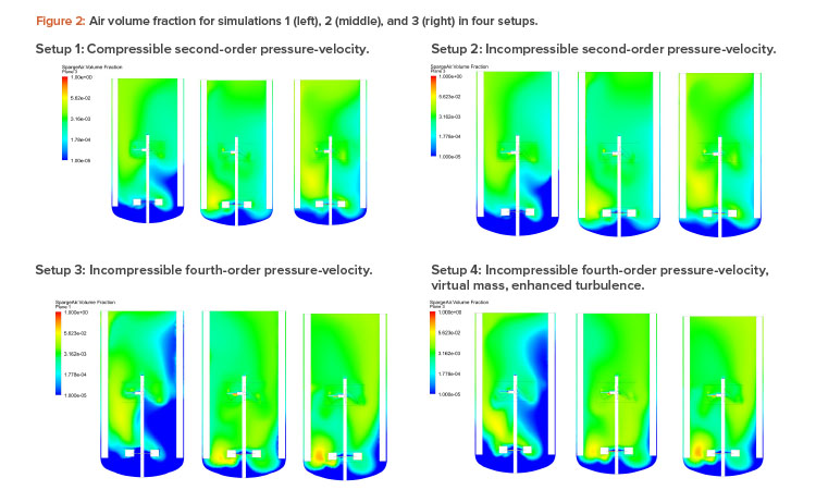
Results
Figures 2 and 3 show the air volume fraction and oxygen transfer rate distributions, respectively, for all final simulations. The differences between the noncompressible and compressible second-order pressure-velocity coupling runs are not as significant as the differences between the fourth-order and second-order pressure-velocity coupling runs. This is not surprising because fourth-order numerics will capture more detail. The air volume fraction figures (Figure 2) show evidence that flooding occurred for simulation 1, which was operating at 25 RPM and 200 NLPM (see Table 2) because the impellers were not properly dispersing the gas phase; regions in blue contained little to no gas.
Convergence
We tracked residuals, various outputs (e.g., forces, Sauter diameter, kLa), and imbalances during the solver run for insight into convergence. Residual root mean square (RMS) levels typically fell below 5E-3 for all equation classes (e.g., momentum, mass, bubble-size fraction), although not all equation classes fell below root mean square values 1E-4. Other researchers encountered similar high residual levels for these types of simulations.2 ,3 ,6 We also used dou-ble precision and found no noticeable improvement for lowering residual values.
We tracked all imbalances, and most equation classes bounced around an imbalance of zero. Typical computational fluid dynamics guidance suggests that all imbalances are less than 1% before a solution can be considered converged; however, for these simulations, this was not possible because it was typical for some equa-tion classes to bounce around at ±5%.
In all the simulations, the steadiness of various output parameters (e.g., forces, kLa, gas holdup) was tracked for a prediction on convergence. A time-step size no larger than 0.01 seconds was used for all final simulations, although one must initially use a much smaller time step (such as 1E-5 sec) to avoid crashing the linear solver. This time step is then steadily increased up to 0.01 seconds as the solution progresses. The time step acts as a relaxation factor for steady-state ANSYS CFX simulations, and one may have to experiment with it for each unique model.
| Simulation No. | Impeller Speed (RPM) |
Sparge Air Rate (NLPM) |
Experimental kLa (hr–1) |
CFD kLa (hr–1) |
% Difference |
|---|---|---|---|---|---|
| Setup 1: Compressible second-order pressure-velocity | |||||
| 1** | 25 | 200 | 4.25 | 4.10 | 3.4 |
| 2** | 38 | 200 | 10.33 | 70.6 | 31.6 |
| 3* | 38 | 400 | 12.43 | 12.43 | 0.0 |
| Setup 2: Incompressible second-order pressure-velocity | |||||
| 1** | 25 | 200 | 4.25 | 4.22 | 0.6 |
| 2** | 38 | 200 | 10.33 | 7.14 | 30.8 |
| 3* | 38 | 400 | 12.43 | 12.43 | 0.0 |
| Setup 3: Incompressible fourth-order pressure-velocity | |||||
| 1** | 25 | 200 | 4.25 | 4.14 | 2.4 |
| 2** | 38 | 200 | 10.33 | 9.47 | 8.3 |
| 3* | 38 | 400 | 12.43 | 12.43 | 0.0 |
| Setup 4: Incompressible fourth-order pressure-velocity, virtual mass, enhanced turbulence | |||||
| 1** | 25 | 200 | 4.25 | 4.06 | 4.5 |
| 2** | 38 | 200 | 10.33 | 9.47 | 8.3 |
| 3* | 38 | 400 | 12.43 | 12.43 | 0.0 |
| New bioreactor using setup 4 | |||||
| 1* | 41 | 250 | 5.76 | 5.76 | 0.0 |
| 2** | 28 | 158 | 2.27 | 2.18 | 4.0 |
| 3** | 28 | 250 | 4.35 | 3.68 | 15.4 |
| 4** | 28 | 333 | 5.90 | 4.97 | 15.9 |
*Benchmarked case
**Predicted case
Discussion
Because only kLa experimental results were available, this was the only parameter that was compared between computational fluid dynamics simulations and experimental data. Simulation 3 was used as the benchmarking case to adjust the kLa constant so its kLa matched experimental data. Benchmarking required for the kLa constant to be updated from 0.4 to 0.53 for setup 1, from 0.4 to 0.58 for setup 2, from 0.4 to 0.53 for setup 3, and from 0.4 to 0.50 for setup 4.
After discovering setup 4 (i.e., incompressible, fourth-order pressure-velocity coupling, virtual mass, enhanced turbulence) provided for the most accurate results, we applied this setup to a completely different bioreactor, which had a different working volume, dual-pitched blade impellers, and a different gas sparger design. A mesh independence study for this bioreactor was not performed. Instead, this bioreactor was meshed with a total of 2,548,980 elements using a similar mesh-sizing approach as the previous bioreactor model. The bottom impeller volume was meshed with 563,407 elements, the top impeller volume was meshed with 591,214 elements, and the vessel was meshed with 1,394,359 elements. The predicted results were similar in that kLa was predicted accurately (within 16%), this time using a kLa constant of 0.4 from the benchmarked case. Table 2 shows the computational fluid dynamics versus experimental data for both bioreactors.
As can be seen in Table 2, computational fluid dynamics correctly predicted the kLa trend with setup 4, with the best agreement against experimental data (within 16%). Further, computational fluid dynamics visually illustrated the local kLa and gas fractions, providing valuable insight into potential design and process improvements.
Conclusion
The difference between the compressible and incompressible second-order models was minor, with the incompressible model providing slightly better results with experimental data. This result is counterintuitive because the air bubbles change density as they travel toward the free surface. The incompressible fourth-order pressure-velocity coupling models offered a better comparison against experimental data, with the virtual mass and enhanced turbulence (Sato) model predicting results within 16% of experimental data, tested on two different bioreactors; however, computational fluid dynamics underpredicted kLa.
Although experimental data were used for benchmarking, applying this method (i.e., setup 4) does not require experimental data if the purpose is to determine what operating conditions (i.e., impeller speed and sparge rate) will maximize mass transfer for a fixed-system geometry. One can just use a kLa constant of 0.4 (or any other reasonable value) to gauge the relative difference in performance between operating conditions. The method described here shows that good computational fluid dynamics results are achieved even for a flooding scenario and with high residual values, as long as the various variables of interest have shown a plateau.
The results of this study demonstrate that computational fluid dynamics can be valuable for predicting bioreactor mass transfer performance and for optimization purposes, provided the model is setup appropriately.
- 1Talaia, M. A. R. “Terminal Velocity of a Bubble Rise in a Liquid Column.” World Academy of Science, Engineering and Technology International Journal of Physical and Mathematical Sciences 1, no. 4 (2007): 220–224.
- 2 a b c Ranganathan, P., and S. Sivaraman. “Investigations on Hydrodynamics and Mass Transfer in Gas–Liquid Stirred Reactor Using Computational Fluid Dynamics.” Chemical Engineering Science 66, no. 14 (2011): 3108–3124. doi:10.1016/j.ces.2011.03.007
- 3 a b c d Sarkar, J., L. K. Shekhawat, V. Loomba, and A. S. Rathore. “CFD of Mixing of Multi-Phase Flow in a Bioreactor Using Population Balance Model.” Biotechnology Progress 32, no. 3 (2016): 613–628. doi:10.1002/btpr.2242
- 44. Taniguchi, S., S. Kawaguchi, and A. Kikuchi. “Fluid Flow and Gas-Liquid Mass Transfer in Gas-Injected Vessel.” Presented at the Second International Conference on CFD in the Materials and Process Industries. CSIRO, Melbourne Australia. 6–8 December 1999.
- 5Petitti, M., M. Vanni, D. L. Marchisio, A. Buffo, and F. Podenzani. “Simulation of Coalescence, Break-up and Mass Transfer in a Gas–Liquid Stirred Tank with CQMOM.” Chemical Engineering Journal 228 (2013): 1182–1194. doi:10.1016/j.cej.2013.05.047
- 6 a b Aubin, J., D. F. Fletcher, and C. Xuereb. “Modeling Turbulent Flow in Stirred Tanks with CFD: The Influence of the Modeling Approach, Turbulence Model and Numerical Scheme.” Experimental Thermal and Fluid Science 2, no. 5 (2004): 431–445. doi:10.1016/j.expthermflusci.2003.04.001
- 7Luo, S. M., and H. Svendsen. “Theoretical Model for Drop and Bubble Breakup in Turbulent Dispersions.” AIChE Journal 42, no. 5 (1996): 1225–1233. doi:10.1002/aic.690420505
- 8Prince, M., and H. Blanch. “Bubble Coalescence and Break-Up in Air-Sparged Bubble Columns.” AIChE Journal 36, no. 10 (1990): 1485–1499. doi:10.1002/aic.690361004
- 9Ishii, M., and N. Zuber. “Drag Coefficient and Relative Velocity in Bubbly, Droplet or Particulate Flows.” AIChE Journal 25, no. 5 (1979): 843–855. doi:10.1002/aic.690250513
- 10Burns, A. D. B., T. Frank, I. Hamill, and J. M. Shi. “The Favre Averaged Drag Model for Turbulent Dispersion in Eulerian Multi-Phase Flows.” Presented at the 5th International Conference on Multiphase Flow, ICMF-2004, Yokohama, Japan.